Content
Ultrasonography Basics
Click on an item to jump to that section.
- Introduction
- Ultrasound wave creation
- Transducer selection
- Ultrasound imaging echogenicities
- Identification of structures
- Scanning planes
- Image optimization
- Needle alignment
- References
Introduction
Ultrasound imaging is a diagnostic medical procedure that uses high-frequency sound waves to produce dynamic images (sonograms) of organs, tissues or blood flow inside the body. The frequency of an ultrasound wave is above 20,000 Hz and that of medical ultrasound is 2.5-15 MHz. Human hearing is in the 20-20,000 Hz range. The speed of sound varies in different biological media, however, the average value is assumed to be 1,540 m/sec for most human soft tissues. The speed of sound can be calculated by multiplying wavelength to frequency. Thus sound with a high frequency has a short wavelength and vice versa.
Ultrasound wave creation
An ultrasound wave is generated when an electric field is applied to an array of piezoelectric crystals located on the transducer surface. Electrical stimulation causes mechanical distortion of the crystals resulting in vibration and production of sound waves. The sound waves emitted from the transducer are transmitted into the body, reflected off the tissue interface and returned to the transducer. These are then converted into an electric signal, which is processed and displayed as an image on the screen. The conversion of sound to electrical energy is called the piezoelectric effect.
Transducer selection
The first step in the systematic scanning process is to select an appropriate transducer. This depends upon the depth and the location of the area to be scanned (Figure 1).
- High frequency (7-15 mHz) (linear) transducer has higher resolution but poor penetration. It is useful for peripheral nerve blocks and central venous cannulation as these structures are superficially located.
- Low frequency (2-5 mHz) (curved array) transducer has lower resolution but better penetration. This is useful for epidural/spinal blocks as these structures are deeply situated.
An orientation marker is usually located on the side of the ultrasound transducer. It helps to orient the image on the screen with respect to the patient position (Figure 1).
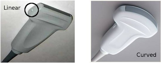
Figure 1. Different types of transducers. Linear (left); Curved (right). The orientation marker on the linear transducer is marked with a circle.
Ultrasound imaging echogenicities
Different structures emit different signals on ultrasound imaging, which are termed as echogenicities. Hyperechoic structures appear white and bright on the ultrasound image, while isoechoic have the same density as the surrounding structures and appear grey. Hypoechoic structures appear dark, black and produce a weak signal (Figure 2).
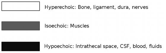
Figure 2. Examples of different ultrasound echogenicities.
Identification of structures
Different structures can be identified based on their anatomical location, shape and echogenic pattern. The examples of blood vessels, nerves, bones and ligaments are given below:
- Blood vessels: Veins and arteries, in the transverse view, appear as circular hypoechoic structures surrounded by hyperechoic rims. Arteries can be easily identified by their pulsatile nature. Veins collapse with the pressure of the ultrasound probe while the arteries remain stiff (Figure 3).
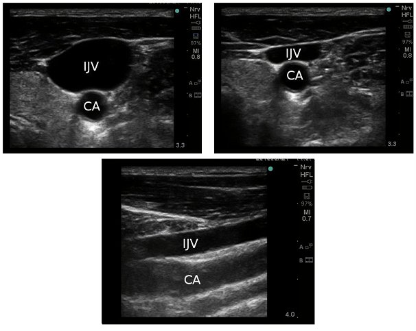
Figure 3. Top: Internal jugular vein (IJV) and carotid artery (CA) in the transverse view with the transducer held on the skin without pressure (left) and with pressure (right). Note that with pressure, IJV appears compressed while the CA has retained its shape. Bottom: These blood vessels in the longitudinal plane.
- Nerves: Nerves below the clavicle and in the lower limbs are predominantly hyperechoic and have a honey comb appearance. The degree of hyperechogenicity likely reflects the amount of connective tissue within the nerve. In the longitudinal view, they appear as hypoechoic longitudinal elements (fascicle groups) interspersed with hyperechoic perineural connective tissues (Figure 4).
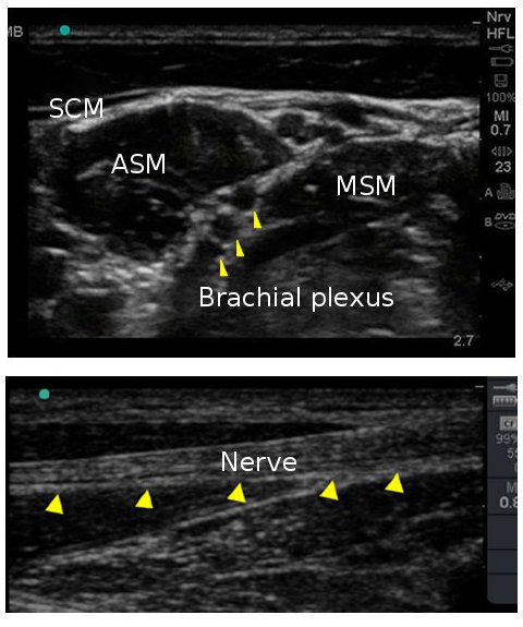
Figure 4. Top: Interscalene brachial plexus in transverse view. Bottom: A nerve in longitudinal plane. Note the honeycomb appearance of nerves represented by arrowheads in both planes. (SCM=sternocleidomastoid; ASM=anterior scalene muscle; MSM=middle scalene muscles).
- Ligaments and Bones: These appear hyperechoic on the ultrasound image. However, bone has high acoustic impedance and does not allow the sound waves to pass through it. This produces a hypoechoic shadow underneath intensely hyperechoic bony structure, termed as Acoustic shadow. Hence while scanning through bony structures, it is necessary to find Acoustic window, an area through which sound waves can be transmitted to visualize the deeper structures (Figure 5).
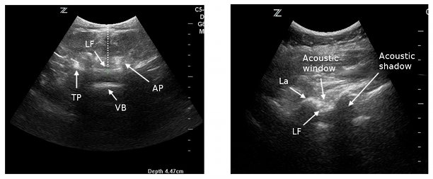
Figure 5. Left: Ultrasound view of the lumbar spine in transverse plane. Right: Ultrasound image of the lumbar spine in longitudinal plane with acoustic windows between lamina and acoustic shadows under lamina. (LF=ligamentum flavum; VB=vertebral body; AP=articulate process; TP=transverse process; La=lamina).
Scanning planes
Scanning in different planes or axes helps in identification of the structures more accurately and facilitates the location and needling of the target areas. Longitudinal axis usually refers to scanning in a plane parallel to the structures while transverse axis refers to scanning in a plane perpendicular to the structures (Figure 6).
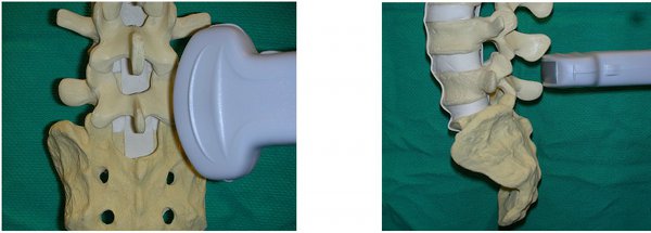
Figure 6. Scanning in longitudinal (left) and transverse (right) planes.
Image optimization
Fine movements of the transducer can help in obtaining the best image.
- Depth settings: Adjust the depth of the image for optimal resolution so that the area of interest is centered on the screen. For scanning for the superficial nerve blocks, set the depth up to 5 cm, while for neuraxial scanning, set it up to 13 cm.
- Gain settings: Adjust gain settings to allow amplification or reduction of intensity of echo. a) Increased gain=brighter image display; b) Decreased gain=darker image display. You can change the gain settings of the entire image (overall) or of any particular field such as near field, or far field. Usually setting the gain to "optimum", provides an appropriate image display.
Needle alignment
This refers to real-time scanning while performing the nerve blocks. For lumbar spine, we do pre-puncture scanning.
In-plane needle alignment (longitudinal, long-axis): In-plane needle alignment refers to aligning the needle with the long-axis of the transducer (along the ultrasound beam) so that the entire shaft and tip of the needle are visible. One of the disadvantages of the in-plane needle view is that, it is easy to lose the image with a slight movement of the transducer as the ultrasound beam is thin. This technique requires excellent hand-eye coordination. It is a preferred technique for Transversus Abdominus Plane block (Figure 7).
Out-of-plane alignment (transverse or short axis): This refers to when the transducer and the needle are perpendicular to each other. It is important to slide the transducer along the shaft of the needle to identify the needle tip. Both the needle tip and shaft in cross section appear as a hyperechoic white dot on the screen. Since only the needle tip is observed as a bright dot, it is sometimes difficult to accurately observe the needle during advancement. Despite this, it is an easier approach for peripheral nerve blocks and central venous cannulation (Figure 7).
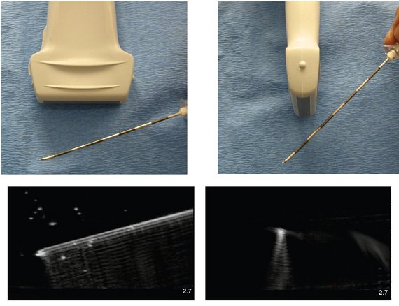
Figure 7. In in-plane technique (left), needle is aligned in the plane of thin ultrasound beam allowing the visualization of the entire shaft and the tip. In out-of plane technique (right), the ultrasound beam transects the needle, and the needle tip or the shaft is observed as a bright spot in the image.
References
- Balki M, Lee Y, Halpern S, Carvalho JCA. Ultrasound imaging of the lumbar spine in the transverse plane: The correlation between estimated and actual depth to the epidural space in obese parturients. Anesthesia Analgesia 2009; 108: 1876-1881.
- Carvalho JCA. Ultrasound facilitated epidurals and spinals in obstetrics. Anesthesiology Clin 2008; 26: 145-158.
- Grau T. The evaluation of ultrasound imaging for neuraxial anesthesia. Can J Anesth 2003; 50: 6 pp R1-R8.
- Grau T. Ultrasonography in the current practice of regional anaesthesia Best Practice & Research. Clinical Anaesthesiology 2005; 19: 175–200.
- http://www.usra.ca/